Exponential Lifetime Model

Introduction

The exponential_lifetime model is a reference implementation demonstrating how to build a specialized likelihood model with:

Closed-form MLE: The fit() method computes the MLE directly as , bypassing optim entirely.
Analytical derivatives: Score, Hessian, and Fisher information matrix in closed form.
Right-censoring: Natural handling via the sufficient statistic .
rdata() method: For Monte Carlo validation and bootstrap studies.

The log-likelihood for Exponential() data with right-censoring is:

where is the number of exact (uncensored) observations and is the total observation time (sum of all times, whether censored or not).

library(likelihood.model)

Uncensored Data

The simplest case: all observations are exact.

set.seed(42)
true_lambda <- 2.5
df <- data.frame(t = rexp(200, rate = true_lambda))

model <- exponential_lifetime("t")
assumptions(model)
#> [1] "independent"              "identically distributed" 
#> [3] "exponential distribution"

Closed-Form MLE

Unlike most models that require optim, the exponential model computes the MLE directly. No initial guess is needed:

mle <- fit(model)(df)

cat("MLE:", coef(mle), "(true:", true_lambda, ")\n")
#> MLE: 2.159 (true: 2.5 )
cat("SE:", se(mle), "\n")
#> SE: 0.1527
cat("95% CI:", confint(mle)[1, ], "\n")
#> 95% CI: 1.86 2.458
cat("Score at MLE:", score_val(mle), "(exactly zero by construction)\n")
#> Score at MLE: 0 (exactly zero by construction)

How the Closed-Form MLE Works

The MLE is for uncensored data. We can verify this against the manual calculation:

n <- nrow(df)
total_time <- sum(df$t)
manual_mle <- n / total_time

cat("fit() result:   ", coef(mle), "\n")
#> fit() result:    2.159
cat("Manual n/T:     ", manual_mle, "\n")
#> Manual n/T:      2.159
cat("Match:", all.equal(unname(coef(mle)), manual_mle), "\n")
#> Match: TRUE

Right-Censored Data

In reliability and survival analysis, observations are often right-censored: we know the item survived past a certain time, but not when it actually failed.

set.seed(42)
true_lambda <- 2.0
censor_time <- 0.5

# Generate latent failure times
x <- rexp(300, rate = true_lambda)
censored <- x > censor_time

df_cens <- data.frame(
  t = pmin(x, censor_time),
  status = ifelse(censored, "right", "exact")
)

cat("Sample size:", nrow(df_cens), "\n")
#> Sample size: 300
cat("Censoring rate:", round(mean(censored) * 100, 1), "%\n")
#> Censoring rate: 41.7 %
cat("Exact observations (d):", sum(!censored), "\n")
#> Exact observations (d): 175
cat("Total time (T):", round(sum(df_cens$t), 2), "\n")
#> Total time (T): 100.8

Fitting with Censoring

model_cens <- exponential_lifetime("t", censor_col = "status")
assumptions(model_cens)
#> [1] "independent"                     "identically distributed"        
#> [3] "exponential distribution"        "non-informative right censoring"

mle_cens <- fit(model_cens)(df_cens)

cat("\nMLE:", coef(mle_cens), "(true:", true_lambda, ")\n")
#> 
#> MLE: 1.737 (true: 2 )
cat("SE:", se(mle_cens), "\n")
#> SE: 0.1313
cat("95% CI:", confint(mle_cens)[1, ], "\n")
#> 95% CI: 1.48 1.994

Ignoring Censoring Leads to Bias

A common mistake is to treat censored times as if they were exact observations. This biases the rate estimate upward (equivalently, the mean lifetime downward):

# Wrong: treat all observations as exact
model_wrong <- exponential_lifetime("t")
mle_wrong <- fit(model_wrong)(df_cens)

cat("Comparison:\n")
#> Comparison:
cat("  True lambda:          ", true_lambda, "\n")
#>   True lambda:           2
cat("  MLE (correct):        ", coef(mle_cens), "\n")
#>   MLE (correct):         1.737
cat("  MLE (ignoring censor):", coef(mle_wrong), "\n")
#>   MLE (ignoring censor): 2.978
cat("\nIgnoring censoring overestimates the failure rate!\n")
#> 
#> Ignoring censoring overestimates the failure rate!

Analytical Derivatives

The model provides score and Hessian in closed form, which we can verify against numerical differentiation:

set.seed(99)
df_small <- data.frame(t = rexp(50, rate = 3))
model_small <- exponential_lifetime("t")
lambda_test <- 2.5

# Analytical score
score_fn <- score(model_small)
analytical_score <- score_fn(df_small, lambda_test)

# Numerical score (via numDeriv)
ll_fn <- loglik(model_small)
numerical_score <- numDeriv::grad(
  function(p) ll_fn(df_small, p), lambda_test
)

cat("Score at lambda =", lambda_test, ":\n")
#> Score at lambda = 2.5 :
cat("  Analytical:", analytical_score, "\n")
#>   Analytical: 1.889
cat("  Numerical: ", numerical_score, "\n")
#>   Numerical:  1.889
cat("  Match:", all.equal(unname(analytical_score), numerical_score), "\n")
#>   Match: TRUE

# Analytical Hessian
hess_fn <- hess_loglik(model_small)
analytical_hess <- hess_fn(df_small, lambda_test)

numerical_hess <- numDeriv::hessian(
  function(p) ll_fn(df_small, p), lambda_test
)

cat("\nHessian at lambda =", lambda_test, ":\n")
#> 
#> Hessian at lambda = 2.5 :
cat("  Analytical:", analytical_hess[1, 1], "\n")
#>   Analytical: -8
cat("  Numerical: ", numerical_hess[1, 1], "\n")
#>   Numerical:  -8
cat("  Match:", all.equal(analytical_hess[1, 1], numerical_hess[1, 1]), "\n")
#>   Match: TRUE

Fisher Information Matrix

The expected Fisher information for Exponential() is . The model provides this analytically:

fim_fn <- fim(model_small)
n_obs <- nrow(df_small)
lambda_hat <- coef(fit(model_small)(df_small))

fim_analytical <- fim_fn(lambda_hat, n_obs)

cat("FIM at MLE (lambda =", lambda_hat, "):\n")
#> FIM at MLE (lambda = 2.761 ):
cat("  Analytical n/lambda^2:", n_obs / lambda_hat^2, "\n")
#>   Analytical n/lambda^2: 6.56
cat("  fim() result:         ", fim_analytical[1, 1], "\n")
#>   fim() result:          6.56
cat("  Match:", all.equal(n_obs / unname(lambda_hat)^2, fim_analytical[1, 1]), "\n")
#>   Match: TRUE

Fisherian Likelihood Inference

The package supports pure likelihood-based inference. Instead of confidence intervals (which make probability statements about parameters), likelihood intervals identify the set of parameter values that are “well supported” by the data.

set.seed(42)
df_fish <- data.frame(t = rexp(100, rate = 2.0))
model_fish <- exponential_lifetime("t")
mle_fish <- fit(model_fish)(df_fish)

# Support function: S(lambda) = logL(lambda) - logL(lambda_hat)
# Support at MLE is always 0
s_mle <- support(mle_fish, coef(mle_fish), df_fish, model_fish)
cat("Support at MLE:", s_mle, "\n")
#> Support at MLE: 0

# At a different value, support is negative
s_alt <- support(mle_fish, c(lambda = 1.5), df_fish, model_fish)
cat("Support at lambda=1.5:", s_alt, "\n")
#> Support at lambda=1.5: -1.375

# Relative likelihood: R(lambda) = L(lambda)/L(lambda_hat) = exp(S)
rl_alt <- relative_likelihood(mle_fish, c(lambda = 1.5), df_fish, model_fish)
cat("Relative likelihood at lambda=1.5:", rl_alt, "\n")
#> Relative likelihood at lambda=1.5: 0.253

Likelihood Intervals

A 1/k likelihood interval contains all where . The 1/8 interval is roughly analogous to a 95% confidence interval:

li <- likelihood_interval(mle_fish, df_fish, model_fish, k = 8)
print(li)
#> 1/8 Likelihood Interval (R >= 0.125)
#> -----------------------------------
#>        lower upper
#> lambda  1.44 2.167
#> attr(,"k")
#> [1] 8
#> attr(,"relative_likelihood_cutoff")
#> [1] 0.125

cat("\nWald 95% CI for comparison:\n")
#> 
#> Wald 95% CI for comparison:
print(confint(mle_fish))
#>        2.5% 97.5%
#> lambda 1.43 2.128

Profile Log-Likelihood

prof <- profile_loglik(mle_fish, df_fish, model_fish, param = 1, n_grid = 100)

plot(prof$lambda, prof$support, type = "l", lwd = 2,
     xlab = expression(lambda), ylab = "Support",
     main = "Profile Support Function")
abline(h = -log(8), lty = 2, col = "red")
abline(v = coef(mle_fish), lty = 3, col = "blue")
legend("topright",
       legend = c("Support S(lambda)", "1/8 cutoff", "MLE"),
       lty = c(1, 2, 3), col = c("black", "red", "blue"), lwd = c(2, 1, 1))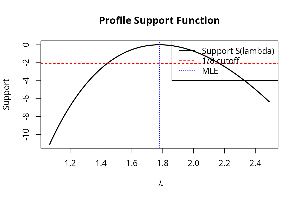

Monte Carlo Validation with `rdata()`

The rdata() method generates synthetic data from the model, enabling Monte Carlo studies. Here we verify that the MLE is unbiased and that the asymptotic standard error matches the empirical standard deviation:

set.seed(42)
true_lambda <- 3.0
n_obs <- 100
n_sim <- 1000

model_mc <- exponential_lifetime("t")
gen <- rdata(model_mc)

# Simulate n_sim datasets and fit each
mle_vals <- replicate(n_sim, {
  sim_df <- gen(true_lambda, n_obs)
  coef(fit(model_mc)(sim_df))
})

cat("Monte Carlo results (", n_sim, "simulations, n=", n_obs, "):\n")
#> Monte Carlo results ( 1000 simulations, n= 100 ):
cat("  True lambda:       ", true_lambda, "\n")
#>   True lambda:        3
cat("  Mean of MLEs:      ", mean(mle_vals), "\n")
#>   Mean of MLEs:       3.038
cat("  Bias:              ", mean(mle_vals) - true_lambda, "\n")
#>   Bias:               0.03775
cat("  Empirical SE:      ", sd(mle_vals), "\n")
#>   Empirical SE:       0.3182
cat("  Theoretical SE:    ", true_lambda / sqrt(n_obs), "\n")
#>   Theoretical SE:     0.3
cat("  (SE = lambda/sqrt(n) from Fisher information)\n")
#>   (SE = lambda/sqrt(n) from Fisher information)

Cross-Validation with `likelihood_name("exp")`

The analytical model should produce the same log-likelihood as the generic distribution-wrapping approach:

set.seed(42)
df_cv <- data.frame(t = rexp(100, rate = 2.0))

model_analytical <- exponential_lifetime("t")
model_generic <- likelihood_name("exp", ob_col = "t",
                                  censor_col = "censor")

# Need a censor column for likelihood_name
df_cv_generic <- data.frame(t = df_cv$t, censor = rep("exact", 100))

lambda_test <- 2.3
ll_analytical <- loglik(model_analytical)(df_cv, lambda_test)
ll_generic <- loglik(model_generic)(df_cv_generic, lambda_test)

cat("Log-likelihood at lambda =", lambda_test, ":\n")
#> Log-likelihood at lambda = 2.3 :
cat("  Analytical model:", ll_analytical, "\n")
#>   Analytical model: -46
cat("  Generic model:   ", ll_generic, "\n")
#>   Generic model:    -46
cat("  Match:", all.equal(ll_analytical, ll_generic), "\n")
#>   Match: TRUE

Summary

The exponential_lifetime model demonstrates several design patterns available in the likelihood.model framework:

Feature	How it’s implemented
Closed-form MLE	Override `fit()` to return `fisher_mle` directly
Analytical derivatives	Implement `score()`, `hess_loglik()`, `fim()`
Right-censoring	Sufficient statistics handle censoring naturally
Data generation	`rdata()` method for Monte Carlo validation
Fisherian inference	Works out of the box via `support()`, `likelihood_interval()`, etc.

These patterns apply to any distribution where you want tighter integration than likelihood_name() provides. See weibull_uncensored for another example with analytical derivatives (but without a closed-form MLE).

Session Info

sessionInfo()
#> R version 4.3.3 (2024-02-29)
#> Platform: x86_64-pc-linux-gnu (64-bit)
#> Running under: Ubuntu 24.04.3 LTS
#> 
#> Matrix products: default
#> BLAS:   /usr/lib/x86_64-linux-gnu/blas/libblas.so.3.12.0 
#> LAPACK: /usr/lib/x86_64-linux-gnu/lapack/liblapack.so.3.12.0
#> 
#> locale:
#>  [1] LC_CTYPE=C.UTF-8       LC_NUMERIC=C           LC_TIME=C.UTF-8       
#>  [4] LC_COLLATE=C.UTF-8     LC_MONETARY=C.UTF-8    LC_MESSAGES=C.UTF-8   
#>  [7] LC_PAPER=C.UTF-8       LC_NAME=C              LC_ADDRESS=C          
#> [10] LC_TELEPHONE=C         LC_MEASUREMENT=C.UTF-8 LC_IDENTIFICATION=C   
#> 
#> time zone: America/Chicago
#> tzcode source: system (glibc)
#> 
#> attached base packages:
#> [1] stats     graphics  grDevices utils     datasets  methods   base     
#> 
#> other attached packages:
#> [1] likelihood.model_0.9.1
#> 
#> loaded via a namespace (and not attached):
#>  [1] cli_3.6.5            knitr_1.50           rlang_1.1.7         
#>  [4] xfun_0.54            generics_0.1.4       textshaping_1.0.4   
#>  [7] jsonlite_2.0.0       htmltools_0.5.8.1    ragg_1.5.0          
#> [10] sass_0.4.10          rmarkdown_2.30       evaluate_1.0.5      
#> [13] jquerylib_0.1.4      MASS_7.3-60.0.1      fastmap_1.2.0       
#> [16] numDeriv_2016.8-1.1  yaml_2.3.11          mvtnorm_1.3-3       
#> [19] lifecycle_1.0.5      algebraic.mle_0.9.0  compiler_4.3.3      
#> [22] fs_1.6.6             htmlwidgets_1.6.4    algebraic.dist_0.1.0
#> [25] systemfonts_1.3.1    digest_0.6.39        R6_2.6.1            
#> [28] bslib_0.9.0          tools_4.3.3          boot_1.3-32         
#> [31] pkgdown_2.2.0        cachem_1.1.0         desc_1.4.3